The minimum connector problem gives a way to join every vertex in a network so that the total weight of the edges used is minimised.
Figure 1: Roads connecting towns in southern England
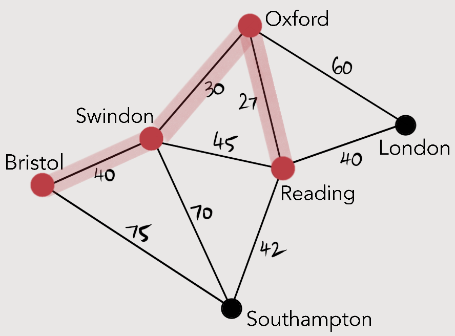
The towns in southern England are to be connected with a new fibre-optic cable system. The hub of the system is to be in London. What is the minimum length of cable needed to connect the towns?
There are two algorithms that we can use to solve this type of problem:
Kruskal’s algorithm finds the minimum spanning tree for a network.
Kruskal’s algorithm has the following steps:
Select the edge with the lowest weight that does not create a cycle. If there are two or more edges with the same weight choose one arbitrarily.
Repeat step 1 until the graph is connected and a tree has been formed.
Example
Finding the minimum spanning tree that follows the road network in southern England
Using Kruskal’s algorithm the minimum spanning tree is generated as follows (each selected edge is coloured red). Click or tap an image for a larger view.
Figure 1: Roads connecting towns in southern England
Figure 2: Kruskal solution step 1
Figure 3: Kruskal solution step 2
Figure 4: Kruskal solution step 3
Figure 5: Kruskal solution step 4
Figure 6: Kruskal solution step 5
The solution for the minimum spanning tree contains the edges {(Bristol, Swindon), (Swindon, Oxford), (Oxford, Reading), (Reading, London), (Reading, Southampton)}. The total weight (distance) for the minimum solution is .
Prim’s algorithm generates a minimum spanning tree for a network. Prim’s algorithm has the following steps:
Select any vertex. Connect the nearest vertex.
Find the vertex that is nearest to the current tree but not already connected and connect that.
Repeat step 2 until all vertices are connected.
Often, assuming that you are doing this for the purposes of an exam, you will be told the starting vertex for step 1. If you find that there is more than one vertex equally close in step 2, choose one arbitrarily.
Example
Finding the minimum spanning tree that follows the road network in southern England.
Using Prim’s algorithm the minimum spanning tree is generated as follows (each selected edge and node is coloured red). Click or tap an image for a larger view.
Figure 1: simplified road network of southern England, Swindon selected as a start point.
Figure 2: Prim’s algorithm step 1, connecting Swindon to Oxford, the nearest adjacent node.
Figure 3: Prim’s algorithm step 2, connecting Oxford to Reading, the nearest node not already in the tree.
Figure 4: Prim’s algorithm step 2, connecting Swindon to Bristol, the nearest node not already in the tree. Bristol was chosen arbitrarily at this point, but London is the same distance and could have equally have been chosen.
Figure 5: Prim’s algorithm step 2, connecting Reading to London, the nearest node not already in the tree.
Figure 6: Prim’s algorithm step 2, connecting Reading to Southampton, the nearest node not already in the tree.
The solution contains the following edges {(Bristol, Swindon), (Swindon, Oxford), (Oxford, Reading), (Reading, London), (Reading, Southampton)} and the total weight (distance) for the minimum solution is .
Other points to note
Prim’s Algorithm also has a table-based form that can easily be applied to matrices or distance tables. This means that it is particularly suited for applying to a computerised solution.
Due to the number of comparisons of weight needed at each iteration, Prim’s Algorithm is .
Prim’s algorithm is also suitable for use on distance tables or matrices, or the equivalent for the problem. This is useful for large problems where drawing the network diagram would be hard or time-consuming.
That tables can be used makes the algorithm more suitable for automation than Kruskal’s algorithm. The reason for this is that the data used would have to be sorted to be used with Kruskal’s algorithm. With Prim’s algorithm, however, it is only the minimum value that is of interest, so no sorting is normally necessary.
We will look again at our question that requires a minimum spanning tree for the network of towns in the south of England using main road connections. The network diagram is as shown in figure 1.
Figure 1: Network of road connections in southern England.
The network shown in Figure 1 can be represented by the adjacency matrix shown in Table 1.
Bristol
London
Oxford
Reading
Southampton
Swindon
Bristol
–
×
×
×
75
40
London
×
–
60
40
×
70
Oxford
×
60
–
27
×
30
Reading
×
40
27
–
42
45
Southampton
75
×
×
42
–
70
Swindon
40
70
30
45
70
–
Table 1: tabular version of road network. × means no direct link.
The tabular form of Prim’s algorithms has the following steps:
Select any vertex (town). Cross out its row. Select the shortest distance (lowest value) from the column(s) for the crossed out row(s). Highlight that value.
Cross out the row with the newly highlighted value in. Repeat step 1. Continue until all rows are crossed out.
Once all rows are crossed out, read off the connections. The column and the row of each highlighted value are the vertices that are linked and should be included.
Example
First we will choose a town at random – Swindon – and cross out that row. Then we highlight the smallest value in the column for the crossed out row.
Bristol
London
Oxford
Reading
Southampton
Swindon
Bristol
–
×
×
×
75
40
London
×
–
60
40
×
70
Oxford
×
60
–
27
×
30
Reading
×
40
27
–
42
45
Southampton
75
×
×
42
–
70
Swindon
40
70
30
45
70
–
Table 2: Prim’s algorithm first iteration.
Next we need to cross out the row with the newly-highlighted value in (the Oxford row). Then we look for, and highlight, the smallest value in the columns for the two crossed out rows (Swindon and Oxford).
Bristol
London
Oxford
Reading
Southampton
Swindon
Bristol
–
×
×
×
75
40
London
×
–
60
40
×
70
Oxford
×
60
–
27
×
30
Reading
×
40
27
–
42
45
Southampton
75
×
×
42
–
70
Swindon
40
70
30
45
70
–
Table 3: Prim’s algorithm second iteration.
Next we need to cross out the row with the newly-highlighted value in (the Reading row). Then we look for, and highlight, the smallest value in the columns for the three crossed out rows (Swindon, Oxford, and Reading).
Bristol
London
Oxford
Reading
Southampton
Swindon
Bristol
–
×
×
×
75
40
London
×
–
60
40
×
70
Oxford
×
60
–
27
×
30
Reading
×
40
27
–
42
45
Southampton
75
×
×
42
–
70
Swindon
40
70
30
45
70
–
Table 4: Prim’s algorithm third iteration.
Next we need to cross out the row with the newly-highlighted value in (the Bristol row). Then we look for, and highlight, the smallest value in the columns for the four crossed out rows (Swindon, Oxford, Reading, and Bristol).
Bristol
London
Oxford
Reading
Southampton
Swindon
Bristol
–
×
×
×
75
40
London
×
–
60
40
×
70
Oxford
×
60
–
27
×
30
Reading
×
40
27
–
42
45
Southampton
75
×
×
42
–
70
Swindon
40
70
30
45
70
–
Table 5: Prim’s algorithm fourth iteration.
Next we need to cross out the row with the newly-highlighted value in (the London row). Then we look for, and highlight, the smallest value in the columns for the crossed out rows (Swindon, Oxford, Reading, Bristol, and Southampton).
Bristol
London
Oxford
Reading
Southampton
Swindon
Bristol
–
×
×
×
75
40
London
×
–
60
40
×
70
Oxford
×
60
–
27
×
30
Reading
×
40
27
–
42
45
Southampton
75
×
×
42
–
70
Swindon
40
70
30
45
70
–
Table 6: Prim’s algorithm fifth and final iteration.
We’ve now selected a value from the last undeleted row. This means we’ve selected all the edges that we need to create the minimum spanning tree for the network. All we have left to do is write out the connections between the vertices.
The connections in the network are found by taking the row and column headings for each selected value in the table. The edges are: {(Bristol, Swindon), (London, Reading), (Oxford, Swindon), (Reading, Oxford), (Southampton, Reading)}. This is the set of edges as in the minimum spanning tree generated by the diagrammatic version of the algorithm.
Dijkstra’s algorithm generates the shortest path tree from a given node to any (or every) other node in the network.
Although the problem that we will use as an example is fairly trivial and can be solved by inspection, the technique that we will use can be applied to much larger problems.
Dijkstra’s algorithm requires that each node in the network be assigned values (labels). There is a working label and a permanent label, as well as an ordering label. Whilst going through the steps of the algorithm you will assign a working label to each vertex. The smallest working label at each iteration will become permanent.
The steps of Dijkstra’s algorithm are:
Give the start point the permanent label of 0, and the ordering label 1.
Any vertex directly connected to the last vertex given a permanent label is assigned a working label equal to the weight of the connecting edge added to the permanent label you are coming from. If it already has a working label replace it only if the new working label is lower.
Select the minimum current working value in the network and make it the permanent label for that node.
If the destination node has a permanent label go to step 5, otherwise go to step 2.
Connect the destination to the start, working backwards. Select any edge for which the difference between the permanent labels at each end is equal to the weight of the edge.
It is a good idea to use a system for keeping track of the current working labels and the ordering and permanent labels of each of the nodes in the network. A standard system found on A Level exams is that a small grid is drawn near each of the nodes, working labels are written in the lower box, ordering labels in the upper left box, and permanent labels in the upper right box, as shown in figure 1.
Figure 1: Labelling system for Dijkstra’s Algorithm.
Example
In this example we will consider the network in figure 2. We would like to find the shortest path from node A to node H.
Figure 2: A simple network.The first four steps of the algorithm are completed.
As you can see at the end of the video, the destination node (node H) has a permanent label. This means that a shortest route from A to H has been found.
The shortest route is found by tracing back from the destination node (node H) to the start (node A), selecting each edge for which the difference between permanent values at its terminating nodes is equal to the weight of the edge. The shortest routes for this network are shown in figure 3 below. The edges shown in green (AB and BC) are an alternative to the edge AC shown in red. In this case there are two equivalent shortest routes from A to H.
Figure 3: The shortest routes from A to H in this network.
The solution to the shortest route problem, from A to H, in this network is therefore A-C-G-H, or the equivalent distance A-B-C-G-H. Both have a total distance of 11 units, given by the permanent label of the terminal node.
Prim’s algorithm starts by selecting the least weight edge from one node. In a complete network there are edges from each node.
At step 1 this means that there are comparisons to make.
Having made the first comparison and selection there are unconnected nodes, with a edges joining from each of the two nodes already selected. This means that there are comparisons that need to be made.
Carrying on this argument results in the following expression for the number of comparisons that need to be made to complete the minimum spanning tree:
Dijkstra’s algorithm inspects each of the nodes that have not yet been permanently labelled, so the work per step is approximately proportional to the number of remaining nodes. For the entire process this number is: .
Linear programming is an optimisation technique that will enable you to find a maximum or minimum value for a problem, subject to any constraints that are relevant. In linear programming the constraints and objective function (the thing you are trying to maximise or minimise) are always modelled by linear equations.
There are two things that you need to create in order to be able to solve a linear programming question. First you should use the information given in the question to generate one or more constraint inequalities. Second you need to define the objective function, which describes the problem for which you are trying to find a maximum or minimum.
Before you can do all this you need to define your variables. The variables that you use will depend on the problem. It will be best to work through an example to demonstrate this.
Clive has decided that as a fund-raising activity he will make and sell candles. He has decided to make two types of candle, a plain one, and a scented one. Each candle requires 200g of wax and Clive has bought enough ingredients to make a total of 1.6kg of wax. His idea is to make the scented candles tall and thin, and the plain candles shorter and fatter. This means that the length of wick required for a scented candle is 200mm but only 100mm is needed for a plain candle. Clive only has 1m of wick to use. Clive has worked out from a survey that he won’t be able to sell more scented candles than double the number of plain candles plus three.
If he is going to sell the candles at £3 for a scented candle and £2 for a plain, how many of each should he make so that he raises the most money possible?
Solution
Definitions
The first thing that we must do is define our variables:
Let:
be the number of plain candles made, be the number of scented candles made, and be the income from selling the candles.
Variable definitions
Constraints
Having defined the variables we can construct our constraint inequalities using the information provided in the question. These describe the conditions that will restrict the number of candles that we can make.
The first constraint relates to the mass of wax available. 200g is required for each candle, and the total available is 1.6kg. Converting to consistent units and writing as an inequality, then simplifying we get:
First constraint inequality
The second constraint is given by the amount of wick available and required. 100mm is needed for each plain candle and 200mm is needed for each scented candle. 1m is available. As with the first constraint, we make sure the units are consistent, then write as an inequality and simplify.
Second constraint inequality
The final constraint is that Clive won’t be able to sell more scented candles than double the number of plain candles plus three. Although slightly complicated this constraint can be written as follows:
Third constraint inequality
Trivial constraints
Most linear programming problems will have some constraints that are not explicitly described. Sometimes you will need to infer a constraint from the context; most frequently these will be trivial. Although referred to as trivial, these constraints are important to include. In this case the context means that we are only interested in positive integers:
Trivial constraints
Objective Function
Having constructed all of our constraint inequalities the only thing left for us to do before solving the problem is to generate an objective function. This is created from the information that tells us what we are to optimise (usually make biggest or smallest). In this case, we need to maximise income with each scented candle selling at £3 and each plain candle selling at £2. The objective function will be:
Objective function
Solving the problem graphically
This problem can be solved graphically by constructing the graph below. Using the constraints that we have already constructed:
All of the constraints
Using the coordinates found at or near the vertices in the objective function, we can work out which combination of scented and plain candles will give the greatest income. Because the only solutions that make sense in the context are integer values of both and , it is worth checking coordinate points near the vertices, inside the feasible region.
0
3
2 × 0 + 3 × 3 = £9
0.8
4.6
2 × 0.8 + 3 × 4.6 = £15.40
1
4
2 × 1 + 3 × 4 = £14
6
2
2 × 6 + 3 × 2 = £18
8
0
2 × 8 + 3 × 0 = £16
As you can see, the highest income can be achieved when 6 plain candles and 2 scented candles are sold. This will give an income of £18.
Critical path analysis allows you to determine the best way of arranging activities. The typical question to answer is “what is the minimum time required for a process?”
Performing activities one after the other as you come to them might not be the best way of organising a project. If more than one activity can be worked on at the same time you will need to decide when to start each one. Below, in table 1, are the activities needed to build a house with durations given in days. We are going to perform a critical path analysis on the process of house construction.
Task
Description
Duration
A
Excavate foundations
2
B
Pour concrete
1
C
Build walls
3
D
Construct roof sections
7
E
Put up roof sections
1
F
Tile roof
3
G
Install plumbing
4
H
Install electrics
3
I
Install windows and doors
2
J
Paint ceilings
2
K
Paint walls
3
L
Lay carpets
2
Table 1: Activities involved in building a house
The first thing that we need to do is to decide which of the activities depend on other activities:
B requires that A be complete.
C requires that B be complete.
E requires that C and D be complete.
F requires that E be complete.
G, H, and I all require that F be complete.
J and K require that G, H, and I be complete.
L requires that J and K be complete.
With this information we can draw an activity network. In an activity network the edges represent activities, such as those listed above. The nodes represent events. An event is the start and/or finish of one or more activities. The activity network for the house building example is shown in figure 1.
Figure 1: The activity network for house building.
The activity network shows that there are 12 events involved in the building of this house, and that 12 activities (plus 3 dummy activities) are required before the house is complete.
As you can see, there are a few activities that can occur concurrently. Later we will use this example to find the critical path through the operation (finding a critical path). It is the longest path and determines the minimum length of time that is necessary to complete the house.


 .
.


 .
.


 edges from each node.
 comparisons to make.
 unconnected nodes, with a edges joining from each of the two nodes already selected. This means that there are
  comparisons that need to be made.
 .
. be the number of plain candles made,
  be the number of scented candles made, and
 be the income from selling the candles.


 and
and  , it is worth checking coordinate points near the vertices, inside the feasible region.


