Discrete Maths examples. This branch of mathematics deals with sorting, relationships, optimisation, and game theory amongst many other areas. Now only on the Further Maths Specification that I teach at A Level, this was originally written to support the D1 and D2 modules.
There are two types of graph that exist in mathematics. The first form is the one with which most people are familiar; a representation of a relationship between variables (often x and y) expressed as a line or curve (as in figure 1). An example of the second form of graph is shown in figure 2. This second form represents relationships that are found in discrete mathematics. In discrete mathematics the set of elements is countable and has a one-to-one correspondence with either the set of positive integers, or a subset of the positive integers.
Figure 1: a plot of the function y = (x – 2)² + 1. A function graph as found in continuous mathematics.Figure 2: a graph showing relationships between vertices. A graph from discrete mathematics. Graphs of the sort that we find in discrete mathematics are useful for solving problems concerning configurations and relationships.
Matrix representation of a graph. Elements of the matrix show the number of edges connecting the vertices represented by the row and column of the matrix.
Isomorphic
Graphs are isomorphic if one can be deformed to make the other. The vertices can be moved and the edges straightened or bent to do this.
Planar graph
A graph that can be drawn such that no edges cross.
Bipartite graph (bigraph)
A graph joining two sets. Every edge starts in one set and ends in the other.
Graphs have an order equal to the number of vertices that they contain.
The size of a graph is equal to the number of edges.
Complete graphs have the maximum size for a given order, without loops. For a graph of order the maximum size will be .
The degree of a vertex is equal to the number of edges that enter or leave it.
The maximum vertex degree for a given order, , of graph without loops, is .
The sum of vertex degrees will be double the size of the graph as each edge has two ends. Consequently a graph cannot have an odd number of vertices with an odd degree.
A complete graph is a form of simple graph. Every pair of vertices must be connected by a single edge. Figure 1 shows an example of a complete graph for a set with 6 elements.
A complete graph with vertices is given the notation .
We may need to find out the total number of edges in this graph.
List all the possible pairs of vertices :
AB, AC, AD, AE, AF
BC, BD, BE, BF
CD, CE, CF
DE, DF
EF
Count the number of pairs.
Each pair of vertices must have an edge connecting them so the number of pairs is equal to the number of edges.
Of course, with a set that has many more than 6 elements, you probably wouldn’t want to list all possible pairs. Thankfully there is another, easier way to work out the number of edges in a complete graph. We could calculate the th triangle number. . Remember the binomial coefficient (you might have seen this in your Pure or Statistics lessons).
This binomial coefficient will give you the number of combinations of elements from a set of members.
For this example and .
By using either the formula above, or by counting pairs, we see that the total number of possible pairs in the set is 15. This is the same as the total number of edges in the complete graph for that set.
An Eulerian graph is a connected graph in which each vertex has even order. This means that it is completely traversable without having to use any edge more than once. It is possible to follow an Eulerian cycle starting from any vertex, visiting every other vertex, using all arcs, and returning to the start point without ever repeating an edge. Each vertex will be visited a number of times equal to half its order.
Figure 1. An Eulerian graph with 6 vertices.
Semi-Eulerian Graphs
A semi-Eulerian graph has two vertices of odd order. An Eulerian cycle is not possible, but it is semi-traversable. You can draw the graph starting at one of the vertices with odd order and ending at the other including all of the edges as you go round, without removing your pencil from the paper.
A network is a graph in which one or more edges is assigned a number, called its weight.
Perhaps the easiest way to think of this is to imagine a graph showing the main roads between towns. The number on the edges would normally represent the distance that you have to travel along that road. Figure 1 shows such a network.
Figure 1. Network diagram of road connections between major towns in southern England.
This graph of roads connecting towns in southern England has had the distances in miles added to the edges that represent the routes. This makes the graph a network.
The numbers that correspond to each edge are called weights.
The discrete maths that is included at A Level contains two main applications of networks. These are:
Minimum connector. The tree that connects all of the vertices in the set with the minimum weight when all included edges are summed.
Shortest path The shortest path that connects any two vertices in the set.
The minimum connector problem gives a way to join every vertex in a network so that the total weight of the edges used is minimised.
Figure 1: Roads connecting towns in southern England
The towns in southern England are to be connected with a new fibre-optic cable system. The hub of the system is to be in London. What is the minimum length of cable needed to connect the towns?
There are two algorithms that we can use to solve this type of problem:
Kruskal’s algorithm finds the minimum spanning tree for a network.
Kruskal’s algorithm has the following steps:
Select the edge with the lowest weight that does not create a cycle. If there are two or more edges with the same weight choose one arbitrarily.
Repeat step 1 until the graph is connected and a tree has been formed.
Example
Finding the minimum spanning tree that follows the road network in southern England
Using Kruskal’s algorithm the minimum spanning tree is generated as follows (each selected edge is coloured red). Click or tap an image for a larger view.
Figure 1: Roads connecting towns in southern England
Figure 2: Kruskal solution step 1
Figure 3: Kruskal solution step 2
Figure 4: Kruskal solution step 3
Figure 5: Kruskal solution step 4
Figure 6: Kruskal solution step 5
The solution for the minimum spanning tree contains the edges {(Bristol, Swindon), (Swindon, Oxford), (Oxford, Reading), (Reading, London), (Reading, Southampton)}. The total weight (distance) for the minimum solution is .
Prim’s algorithm generates a minimum spanning tree for a network. Prim’s algorithm has the following steps:
Select any vertex. Connect the nearest vertex.
Find the vertex that is nearest to the current tree but not already connected and connect that.
Repeat step 2 until all vertices are connected.
Often, assuming that you are doing this for the purposes of an exam, you will be told the starting vertex for step 1. If you find that there is more than one vertex equally close in step 2, choose one arbitrarily.
Example
Finding the minimum spanning tree that follows the road network in southern England.
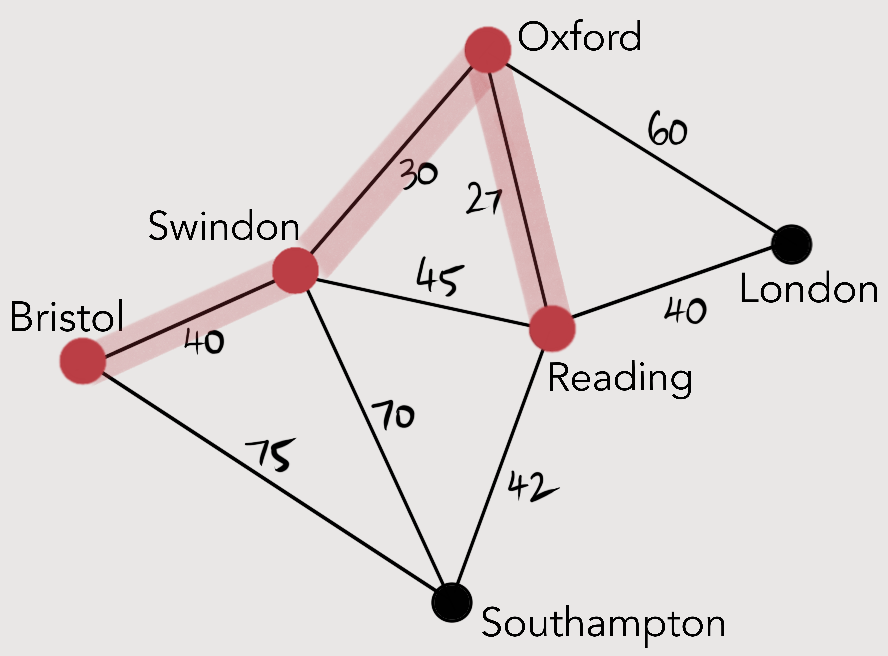
Using Prim’s algorithm the minimum spanning tree is generated as follows (each selected edge and node is coloured red). Click or tap an image for a larger view.
Figure 1: simplified road network of southern England, Swindon selected as a start point.
Figure 2: Prim’s algorithm step 1, connecting Swindon to Oxford, the nearest adjacent node.
Figure 3: Prim’s algorithm step 2, connecting Oxford to Reading, the nearest node not already in the tree.
Figure 4: Prim’s algorithm step 2, connecting Swindon to Bristol, the nearest node not already in the tree. Bristol was chosen arbitrarily at this point, but London is the same distance and could have equally have been chosen.
Figure 5: Prim’s algorithm step 2, connecting Reading to London, the nearest node not already in the tree.
Figure 6: Prim’s algorithm step 2, connecting Reading to Southampton, the nearest node not already in the tree.
The solution contains the following edges {(Bristol, Swindon), (Swindon, Oxford), (Oxford, Reading), (Reading, London), (Reading, Southampton)} and the total weight (distance) for the minimum solution is .
Other points to note
Prim’s Algorithm also has a table-based form that can easily be applied to matrices or distance tables. This means that it is particularly suited for applying to a computerised solution.
Due to the number of comparisons of weight needed at each iteration, Prim’s Algorithm is .
Prim’s algorithm is also suitable for use on distance tables or matrices, or the equivalent for the problem. This is useful for large problems where drawing the network diagram would be hard or time-consuming.
That tables can be used makes the algorithm more suitable for automation than Kruskal’s algorithm. The reason for this is that the data used would have to be sorted to be used with Kruskal’s algorithm. With Prim’s algorithm, however, it is only the minimum value that is of interest, so no sorting is normally necessary.
We will look again at our question that requires a minimum spanning tree for the network of towns in the south of England using main road connections. The network diagram is as shown in figure 1.
Figure 1: Network of road connections in southern England.
The network shown in Figure 1 can be represented by the adjacency matrix shown in Table 1.
Bristol
London
Oxford
Reading
Southampton
Swindon
Bristol
–
×
×
×
75
40
London
×
–
60
40
×
70
Oxford
×
60
–
27
×
30
Reading
×
40
27
–
42
45
Southampton
75
×
×
42
–
70
Swindon
40
70
30
45
70
–
Table 1: tabular version of road network. × means no direct link.
The tabular form of Prim’s algorithms has the following steps:
Select any vertex (town). Cross out its row. Select the shortest distance (lowest value) from the column(s) for the crossed out row(s). Highlight that value.
Cross out the row with the newly highlighted value in. Repeat step 1. Continue until all rows are crossed out.
Once all rows are crossed out, read off the connections. The column and the row of each highlighted value are the vertices that are linked and should be included.
Example
First we will choose a town at random – Swindon – and cross out that row. Then we highlight the smallest value in the column for the crossed out row.
Bristol
London
Oxford
Reading
Southampton
Swindon
Bristol
–
×
×
×
75
40
London
×
–
60
40
×
70
Oxford
×
60
–
27
×
30
Reading
×
40
27
–
42
45
Southampton
75
×
×
42
–
70
Swindon
40
70
30
45
70
–
Table 2: Prim’s algorithm first iteration.
Next we need to cross out the row with the newly-highlighted value in (the Oxford row). Then we look for, and highlight, the smallest value in the columns for the two crossed out rows (Swindon and Oxford).
Bristol
London
Oxford
Reading
Southampton
Swindon
Bristol
–
×
×
×
75
40
London
×
–
60
40
×
70
Oxford
×
60
–
27
×
30
Reading
×
40
27
–
42
45
Southampton
75
×
×
42
–
70
Swindon
40
70
30
45
70
–
Table 3: Prim’s algorithm second iteration.
Next we need to cross out the row with the newly-highlighted value in (the Reading row). Then we look for, and highlight, the smallest value in the columns for the three crossed out rows (Swindon, Oxford, and Reading).
Bristol
London
Oxford
Reading
Southampton
Swindon
Bristol
–
×
×
×
75
40
London
×
–
60
40
×
70
Oxford
×
60
–
27
×
30
Reading
×
40
27
–
42
45
Southampton
75
×
×
42
–
70
Swindon
40
70
30
45
70
–
Table 4: Prim’s algorithm third iteration.
Next we need to cross out the row with the newly-highlighted value in (the Bristol row). Then we look for, and highlight, the smallest value in the columns for the four crossed out rows (Swindon, Oxford, Reading, and Bristol).
Bristol
London
Oxford
Reading
Southampton
Swindon
Bristol
–
×
×
×
75
40
London
×
–
60
40
×
70
Oxford
×
60
–
27
×
30
Reading
×
40
27
–
42
45
Southampton
75
×
×
42
–
70
Swindon
40
70
30
45
70
–
Table 5: Prim’s algorithm fourth iteration.
Next we need to cross out the row with the newly-highlighted value in (the London row). Then we look for, and highlight, the smallest value in the columns for the crossed out rows (Swindon, Oxford, Reading, Bristol, and Southampton).
Bristol
London
Oxford
Reading
Southampton
Swindon
Bristol
–
×
×
×
75
40
London
×
–
60
40
×
70
Oxford
×
60
–
27
×
30
Reading
×
40
27
–
42
45
Southampton
75
×
×
42
–
70
Swindon
40
70
30
45
70
–
Table 6: Prim’s algorithm fifth and final iteration.
We’ve now selected a value from the last undeleted row. This means we’ve selected all the edges that we need to create the minimum spanning tree for the network. All we have left to do is write out the connections between the vertices.
The connections in the network are found by taking the row and column headings for each selected value in the table. The edges are: {(Bristol, Swindon), (London, Reading), (Oxford, Swindon), (Reading, Oxford), (Southampton, Reading)}. This is the set of edges as in the minimum spanning tree generated by the diagrammatic version of the algorithm.


 the maximum size will be
  .
. .
.
 .
. th triangle number.
  . Remember the binomial coefficient (you might have seen this in your Pure or Statistics lessons).
 elements from a set of
  and
and  .
.


 .
.


 .
.